
Unintuitive Probability: Machine Repairs
Table of Contents
The more classes I take in probability, the more I realize how often my intuition breaks for these problems, especially when the Exponential distribution is involved. Today I’ll be explaining a homework problem for Stat150 (Stochastic Processes) showcasing unintuitive behavior regarding exponential distributions. Furthermore, I’ll also show a simulation that backs up these results, along with the code used to generate the simulation.
Problem Statement
Formal Solution
To solve this, we take advantage of the Rewards Theorem (Theorem 3.3 in Durrett; also here for a great explanation). Noting that each characteristic period is the first arrival of either a repair completing (\(\textrm{~ Exp}(\mu)\))or a mistake happening (\(\textrm{~ Exp}(\lambda)\)), the period is then the minimum of the two exponentials, (\(\textrm{~ Exp}(\mu + \lambda)\)). The “reward” here is correctly completing a fix, which can be viewed as an indicator RV that takes \(1\) only on success: \(\mathbb{1}_{t_i = \textrm{repair}}\). Applying the rewards theorem then yields
\[\frac{\textrm{E}[r_i]}{\textrm{E}[t_i]} = \frac{\textrm{E}[\mathbb{1}_{t_i = \textrm{repair}}]}{\textrm{E}[\textrm{Exp}(\mu + \lambda)]} = \mu\]This is somewhat unintuitive! It’s saying that the rate at which machines are repaired is independent of the rate at which the worker is making mistakes!
Intuitive Solution
Now that we have a mathematical result, let’s try to intuit the cause. Conditioning on a mistake happening at some time \(t^*\), two things happen: the repair and mistake processes begin anew. However, we note that even if the mistake didn’t happen at this time, both processes would have begun anew regardless due to the memoryless property of the exponential distribution! This result is a bit astounding; to rephrase, due to the memoryless property of the exponential distribution, the worker’s “time until completion” would have restarted at any time \(t^*\) regardless of whether or not a mistake occurred. This directly means that the expected time until completion cannot depend on anything other than \(\mu\), which leads to our solution.
Simulation Code
To simulate this result, we generate two random vectors of the exponential distributions. Then, we create the times at which the mistakes are made in mistake_times (remembering that mistakes happen independently of repairs). After that, we accumulate times at which the machine is correctly fixed in fix_times. Taking the successive differences of fix_times gives the time between fixes, and plotting these values gives us our result.
using Distributions
using Plots
μ = 1
λ = 3
n = 10000

# Generate random vectors as simulated times
μs = rand(Exponential(μ), n)
λs = rand(Exponential(λ), n*10)

mistake_times = cumsum(λs)

# Times that the machine is actually correctly fixed (ie. before interruption)
fix_times = [0.0]
time = 0.0
λ_index = 1

for repairtime in μs
  global time, λ_index
    if repairtime + time > mistake_times[λ_index] # no fix
        time = mistake_times[λ_index]
        λ_index += 1 # increment fail index
    else # fix
        time += repairtime
        push!(fix_times, time)
    end
end

# Construct animation; animate every 5 timesteps
diffs = diff(fix_times)
anim = @gif for i=1:(length(diffs) ÷ 5)
  vals = diffs[1:i]
  histogram(vals, normalize=:probability) # y1
  vline!([mean(vals)])                    # y2
  vline!([μ])                             # y3
end
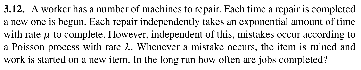
Simulation Results
The orange line y2 is the simulated mean, and the green line y3 is the expected mean (from our math above).
With \(\mu = 1, \lambda = 3\), we get:
and see that our simulated results do indeed match the math.