I’ve never really been a big sports guy, but my brother somehow dragged me into watching the NBA Playoffs. It’s been pretty fun! The series is intense and close, and naturally, I’ve been itching to see if I can wrangle some numbers out of the mess called basketball. Here, I talk a bit about what I did to try to get information out of these numbers, but it’s also a dive into my experience with PyMC3 and Turing.jl.

Warning ahead: All models are wrong, but some are more useful than others. I don’t know if this is one of the useful ones.

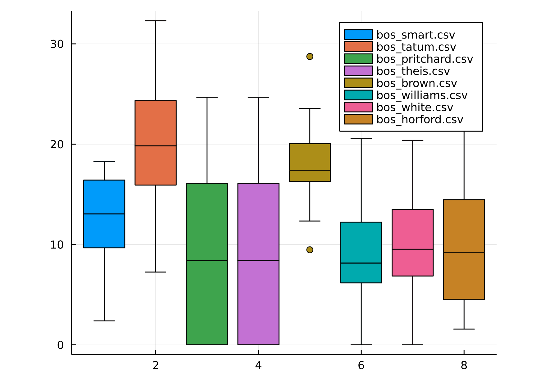
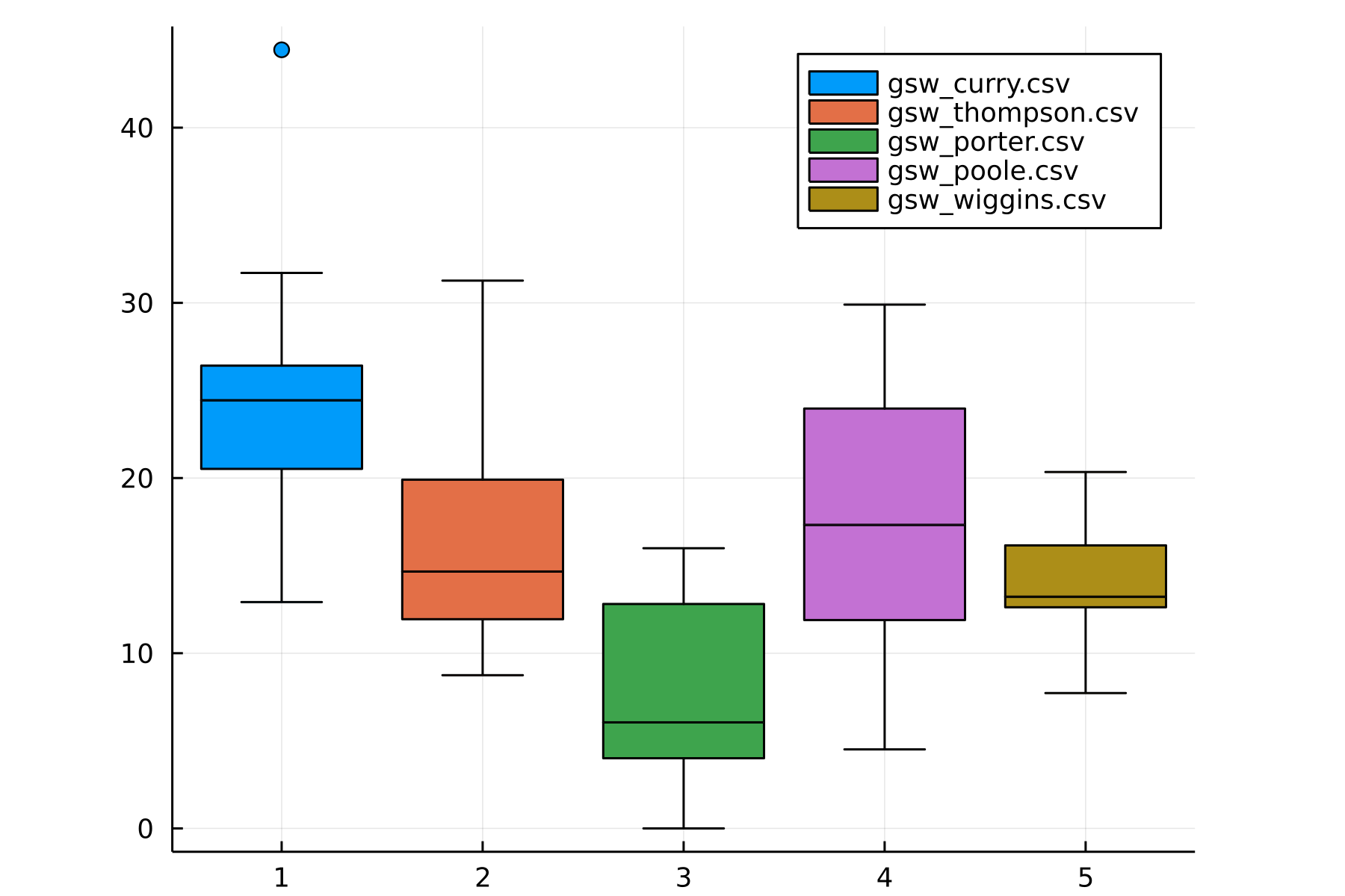
In the first three games, I noticed that Curry was scoring like a madman. Curious to see whether he was scoring far above his usual, I graphed a box-and-whisker plot of the top players’ usual points and eyeballed it. It seems that some players are scoring at their 50-75th percentile range (Curry included), whereas others are scoring at the bottom of their range (Klay). This analysis wasn’t quite that useful, mainly due to one pain point of plotting in Julia: it seems like it’s impossible to overlay scatter points on top of a box-and-whisker plot!¹

Boston Scores:

Warrior Scores:

Seeing this, I left the data alone, and then we watched Game 5.

What an absolutely spectacular game that was! For the first time in forever, Curry didn’t score a single 3 in that game. It piqued my curiosity: I remember a while ago that I read about how hierarchical Bayes models could be used to model game outcomes in Julia, and I was curious if I could do something similar to get the scoring abilities of each player. It wouldn’t be a direct copy-paste of the football simulation for one big reason: instead of modeling a team, I’d be modeling individual players that sum up to a team. Since this was right after my bad experience with Julia above, where the box-and-whisker plot wasn’t very versatile, I wanted to go back to Python. Picking up PyMC, I tried to figure out how to implement such a model.

I spent the next day or so reading up on PyMC and trying to figure out whether I could bend it to my will. The issue with libraries like PyMC is that you have to be very careful with the operations you do; since it’s all just an interface to a lower-level library, there’s a restricted set of operations allowed. For this particular problem, it seems like the two-team problem is solved; the only question was to generalize it to teammates that make up a dynamic team.

The first bright idea that popped up was to construct all permutations of a team as subteams, and then to run the model. There were several issues with this approach. In the most naive way to do this, we would end up throwing away individual players’ contributions. Supposing then we’re a bit smarter, that we encode the teams as a fixed sum of individual random variables and allow the model to update those underlying RVs, we’re still left with the implementation problem: how exactly do you create this many intermediate variables?

I tried researching for a while, but eventually gave up. (In retrospect, I suspect a for loop probably would work, but I’m quite unsure.) It was at this point that I remembered Julia’s Turing.jl library allows for arbitrary Julia expressions, and as I’m moderately familiar with the language, I figured it’d be worth it to give it a second shot.

It turns out that specifying the model wasn’t that difficult! The only point of creativity was to specify 10 inputs to the function (each player playing at a particular time segment) rather than each team. Then, the model boils down to the sum of all of the players on one team subtracted by the sum of the players on the other. For the curious, the relevant lines are here.

And the results!

Attack Values

Interestingly, all defense values are very close to 0. Thinking about it, it makes a lot of sense – when players play round-robin, it’s possible to infer attack-defense values, since we can have rock-paper-scissors situations. However, when it’s a bipartite graph, as with two teams, it’s hard to tease out the reason behind scoring more, whether it’s due to one player having greater attack or due to another having lower defense.

While training this model, I dug into the Turing.ml documentation a bit more. There’s an interesting section on performance tuning. I figured that since my model probably qualifies as a bigger one that I should try :reversediff. Adding that reduced my model training by about a minute, from ~6 minutes to 5. Then, looking into the autodiff section more, I verified that I could memoize the computation, and did so. The training went down to seconds! Wow!

Because of this short time, I had a lot more flexibility to mess with my data and try different things. One thing I glossed over earlier was that the data was partitioned by player time. This means that each data slice tracks only the time 10 players are playing on the court, and stops when any one gets switched out. In my initial analysis, I cut out all samples where the time is less than 60 seconds, since scoring can lead to high variance. (1 points in 1 minute should be viewed as less important than 10 points in 10 minutes.) I tried variations of cutoff times, but it does indeed seem like the noise issue exists. I ended up going back to a 60-second cutoff, and it’s what exists in the repo.

Hopefully this was interesting! If you want to play around with the data and the repo, check it out here.

Footnotes